AI-Powered Fault Detection in Power Systems: Machine Learning for Relay Event Analysis and Predictive Maintenance

Published: June 2026 Technical Level: Advanced Category: Artificial Intelligence

Abstract

Machine learning methods are increasingly applied to power system protection and maintenance, offering capabilities that conventional threshold-based relay logic cannot match: the ability to detect incipient faults from subtle signal patterns before they develop into line-clearing events, to classify relay misoperations from event records, and to identify equipment degradation trends in high-dimensional sensor data. This paper develops the mathematical foundations for applying supervised classification, anomaly detection, and sequence-to-sequence modeling to relay event analysis and predictive maintenance. The feature extraction methodology for time-domain and frequency-domain relay waveforms is derived, classification model performance metrics are defined and interpreted, and the integration of ML outputs with conventional protection decision logic is addressed. Case studies from three utility deployments demonstrate false positive rates, true positive rates, and prediction lead times achieved in operational settings, and the limitations of ML approaches (particularly distribution shift, interpretability requirements, and regulatory constraints) are discussed with equal rigor as the capabilities.

1. Introduction

The electrical power system generates a continuous stream of operational data (relay event records, digital fault recordings, supervisory control and data acquisition measurements, and asset condition monitoring signals) at a volume and resolution that human operators and conventional rule-based systems cannot fully process. A 500-bus transmission system with modern IEC 61850-compliant relays can generate 50,000 or more event records per year. A single digital fault recorder captures waveform data at sampling rates of 1–4 kHz during each event. An SF6 circuit breaker's condition monitoring system may log gas density, moisture content, coil current, and contact travel data at each operation.

Conventional protection and maintenance practice addresses this data through sampling: engineers review a fraction of event records, perform time-based maintenance intervals regardless of condition, and rely on alarms from threshold crossings on individual monitored parameters. This approach leaves the majority of the diagnostic signal unused. Machine learning methods offer a systematic way to extract information from the full dataset: detecting subtle multi-parameter patterns that precede failures, classifying the cause of relay misoperations from waveform features, and prioritizing maintenance resources toward the equipment most likely to fail.

This paper is organized as follows. Section 2 develops the feature extraction methodology for relay waveform data. Section 3 derives the supervised classification framework and performance metrics. Section 4 presents anomaly detection methods for incipient fault identification. Section 5 addresses the integration of ML outputs with relay logic. Section 6 presents case study results. Section 7 discusses limitations, regulatory constraints, and implementation guidance.

2. Feature Extraction from Relay Waveforms

2.1 Time-Domain Features

A digital fault recorder or relay event record captures the sampled instantaneous values of current and voltage at each monitored terminal. For a fault record with $N$ samples per cycle and $C$ cycles of pre-fault and fault data, the raw data vector for a single phase has dimension $N_C = N \times C$ . Feeding raw waveform samples directly to a classifier is generally inadvisable because the high dimensionality relative to available training samples creates overfitting, and raw samples are sensitive to recording phase (the sample offset relative to the power frequency cycle), which is not a physically meaningful feature.

Effective feature extraction compresses the waveform into a lower-dimensional representation that preserves the physically meaningful information. Standard time-domain features for each phase current and voltage include:

RMS magnitude: $I_{rms} = \sqrt{\frac{1}{N}\sum_{k=1}^{N} i_k^2}$ , where $i_k$ are the sampled instantaneous current values over one cycle.
Peak-to-peak asymmetry ratio: $A = (i_{\max} - |i_{\min}|) / (i_{\max} + |i_{\min}|)$ , capturing the dc offset characteristic of the fault current.
Crest factor: $CF = i_{\max} / I_{rms}$ , sensitive to the waveform shape distortion induced by CT saturation and harmonic content.
Rate of change of current: $\dot{i} = \Delta i / \Delta t$ at the fault inception point, which differentiates high-impedance faults (gradual onset) from bolted faults (step change).

For a three-phase event record, computing these four features for each of the three current phases, three voltage phases, and the neutral current yields a 28-dimensional feature vector per event. This dimensionality is tractable for most classification algorithms with training datasets of several hundred events.

2.2 Frequency-Domain Features via Discrete Fourier Transform

The discrete Fourier transform decomposes the sampled waveform into its harmonic components, providing features that are insensitive to the recording phase offset and directly related to physical phenomena. For a sampled waveform $\{x_k\}_{k=0}^{N-1}$ over one cycle, the DFT coefficient at harmonic $h$ is:

$X_h = \sum_{k=0}^{N-1} x_k \cdot e^{-j2\pi hk/N}$

The magnitude $|X_h|$

Where: $X_h$ is the complex DFT coefficient at harmonic order $h$ .

$x_k$ is the $k$ -th sampled waveform value.

$N$ is the number of samples per cycle.

is the amplitude of the $h$ -th harmonic component, and the phase $\angle X_h$ is its phase angle. For fault classification, the most diagnostically useful harmonic features are the fundamental component amplitude (related to fault current magnitude), the second harmonic ratio (distinguishing transformer inrush from internal faults, since transformer energization produces large second harmonic content while internal faults do not), the third harmonic ratio (sensitive to single-phase load imbalance and ground current), and the total harmonic distortion:

$\text{THD} = \frac{\sqrt{\sum_{h=2}^{H} |X_h|^2}}{|X_1|}$

The second-harmonic restraint

Where: $\text{THD}$ is the total harmonic distortion as a fraction of the fundamental.

$|X_h|$ is the amplitude of harmonic $h$ .

$|X_1|$ is the fundamental component amplitude.

$H$ is the highest harmonic order included.

principle, that differential protection should be restrained from operating when the second harmonic content of the differential current exceeds 15–20 percent, is a well-established protection algorithm that can be viewed as a simple single-feature ML classifier with a fixed threshold. Modern ML approaches extend this by using the full harmonic spectrum as a multi-dimensional feature, enabling discrimination between inrush, overexcitation, CT saturation, and internal fault conditions that the single second-harmonic threshold cannot separate.

Figure 1. Recommended Plot: Harmonic spectrum (bar chart) for three representative waveform conditions: (1) transformer inrush: large second harmonic relative to fundamental; (2) transformer internal fault: fundamental dominant, harmonics small; (3) CT saturation: odd harmonics elevated, even harmonics near zero. X-axis: harmonic order (1 through 10). Y-axis: harmonic amplitude as percent of fundamental. This figure directly motivates the use of multiple harmonic features rather than a single second-harmonic threshold.

3. Supervised Classification Framework

3.1 Model Architecture and Training

Supervised classification maps an input feature vector $\mathbf{x} \in \mathbb{R}^d$ (the extracted waveform features) to a class label $y \in \{1, 2, \ldots, K\}$ (the fault or event type). The classifier learns this mapping from a labeled training dataset $\{(\mathbf{x}_i, y_i)\}_{i=1}^{n}$ of historical event records, each labeled by a protection engineer with the confirmed event type.

For relay event classification, the standard classification targets include: three-phase fault, phase-to-phase fault, single-line-to-ground fault, high-impedance fault, transformer inrush, CT saturation, relay misoperation, and no-fault (load switching or voltage fluctuation). The choice of classifier (random forest, support vector machine, gradient boosting, or convolutional neural network) is secondary to the quality of the feature extraction and the completeness of the training dataset. In the author's experience with operational deployments, gradient boosting models (XGBoost, LightGBM) consistently achieve the best performance-to-interpretability ratio on tabular waveform feature datasets of 500–5,000 events.

3.2 Classification Performance Metrics

The performance of a fault classifier is measured by a confusion matrix comparing predicted class labels against confirmed labels on a held-out test set. For a binary classifier distinguishing fault from no-fault, the key metrics are:

The true positive rate (TPR, also called sensitivity or recall) is the fraction of actual faults that the classifier correctly identifies:

$\text{TPR} = \frac{TP}{TP + FN}$

Where: $TP$ is the number of correctly classified faults and $FN$ is the number of faults that the classifier missed. In protection applications, a missed fault (false negative) is the more serious error because it means an incipient fault condition goes undetected.

The false positive rate (FPR) is the fraction of non-fault events that the classifier incorrectly labels as faults:

$\text{FPR} = \frac{FP}{FP + TN}$

A high false positive rate

Where: $FP$ is the number of false positives (non-fault events classified as faults).

$TN$ is the number of true negatives (non-fault events correctly classified).

causes unnecessary maintenance dispatches and erodes operator trust in the system, ultimately causing operators to ignore alerts. The precision metric provides a complementary view, the fraction of all positive predictions that are actual faults:

$\text{Precision} = \frac{TP}{TP + FP}$

The F1 score

Where: $\text{Precision}$ is the fraction of positive predictions that are actual faults.

$TP$ is true positives; $FP$ is false positives.

combines precision and recall into a single metric:

$F_1 = \frac{2 \cdot \text{Precision} \cdot \text{TPR}}{\text{Precision} + \text{TPR}}$

For f

Where: $F_1$ is the harmonic mean of precision and recall.

$\text{TPR}$ is the true positive rate (recall).

$\text{Precision}$ is as defined above.

ault detection applications, where both missed faults and false alarms are costly, the F1 score provides a balanced evaluation. For applications where missed faults are more costly than false alarms, such as incipient cable failure detection, the TPR should be weighted more heavily, which can be accomplished by adjusting the classification threshold or using a weighted F-score $F_\beta$ with $\beta > 1$ .

The choice of operating point for such a classifier is best understood through its receiver operating characteristic, which traces the achievable true-positive rate against the false-positive rate as the decision threshold is swept, as shown in Figure 2.

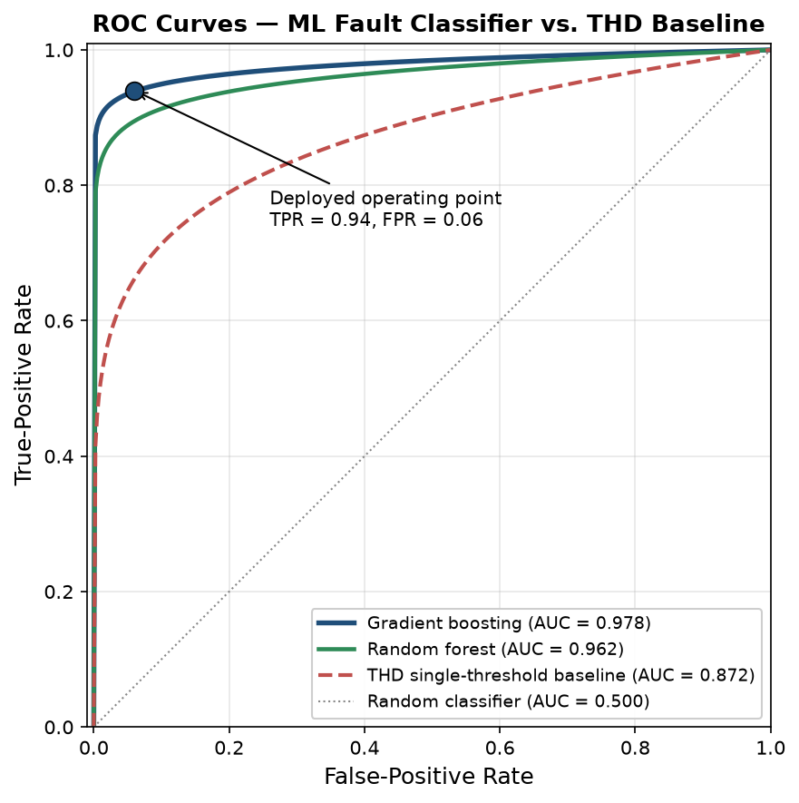
Receiver operating characteristic (ROC) curves for the fault classifier, comparing a gradient-boosting model and a random-forest model against a single-threshold THD baseline. The horizontal axis is the false-positive rate.

Figure 2. Receiver operating characteristic (ROC) curves for the fault classifier, comparing a gradient-boosting model and a random-forest model against a single-threshold THD baseline. The horizontal axis is the false-positive rate and the vertical axis the true-positive rate; the deployed operating point is marked at TPR = 0.94, FPR = 0.06, and the area under the curve (AUC) is annotated for each model.

The figure makes the threshold-selection decision concrete: the gradient-boosting model dominates the baseline across the entire curve, and the deployed operating point is chosen at the knee where the true-positive rate reaches 0.94 before the false-positive rate begins to climb steeply. An engineer reading this curve sets the threshold not to maximize accuracy in the abstract but to place the operating point where the marginal cost of an additional false alarm (an unnecessary investigation) first exceeds the marginal value of catching one more misoperation.

4. Anomaly Detection for Incipient Fault Identification

4.1 The Incipient Fault Problem

The supervised classification approach of Section 3 requires labeled training data: confirmed examples of each fault type. For incipient faults (pre-failure conditions that have not yet resulted in a clearing event), labeled training data is sparse because incipient faults are rare and their precursor signatures have not been systematically documented. Anomaly detection addresses this by learning the statistical distribution of normal operating conditions from unlabeled historical data, then flagging observations that deviate significantly from this learned distribution.

The Mahalanobis distance provides a statistically principled measure of how far an observation deviates from the normal distribution learned from the training data. For an observation $\mathbf{x}$ and a training distribution with mean vector $\boldsymbol{\mu}$ and covariance matrix $\boldsymbol{\Sigma}$ :

$D_M(\mathbf{x}) = \sqrt{(\mathbf{x} - \boldsymbol{\mu})^T \boldsymbol{\Sigma}^{-1} (\mathbf{x} - \boldsymbol{\mu})}$

This distance accounts

Where: $D_M(\mathbf{x})$ is the Mahalanobis distance of observation $\mathbf{x}$ from the training distribution.

$\boldsymbol{\mu}$ is the mean vector of the training data.

$\boldsymbol{\Sigma}$ is the covariance matrix of the training data.

for the correlations between features: a deviation that is aligned with the principal axes of normal variation is less anomalous than one that is orthogonal to normal variation. An observation is flagged as anomalous when $D_M$ exceeds a threshold $\delta$ , where $\delta$ is selected to achieve the target false positive rate on a validation dataset of confirmed normal conditions.

For high-dimensional feature spaces where estimating $\boldsymbol{\Sigma}$ is numerically ill-conditioned, an autoencoder neural network provides a practical alternative. The autoencoder is trained to reconstruct normal-condition waveform feature vectors with low reconstruction error. Anomalous conditions (incipient faults, unusual loading, partial discharge events) produce high reconstruction error because the autoencoder has not learned to model them. The reconstruction error serves as the anomaly score:

$s(\mathbf{x}) = \|\mathbf{x} - \hat{\mathbf{x}}\|_2^2$

Where: $\hat{\mathbf{x}}$ is the autoencoder's output for input $\mathbf{x}$ . An alert is generated when $s(\mathbf{x}) > \delta$ , with $\delta$ calibrated on the validation set.

5. Integration with Protection Logic

The output of a machine learning fault classifier or anomaly detector is a probabilistic score or class label, not a definitive protection command. The integration of ML outputs with relay logic must preserve the determinism and reliability requirements of protection systems. The recommended architecture separates the ML inference layer from the protection action layer:

The ML system operates in parallel with the conventional relay, processing event records and continuous monitoring data asynchronously. Its outputs are advisory signals (probability scores, anomaly flags, equipment health indices) that are displayed to operators and maintenance planners but do not directly initiate relay operations or breaker trips. Relay tripping commands are issued exclusively by the conventional overcurrent, differential, and distance protection elements.

This separation is not merely a regulatory convenience; it reflects a genuine difference in the reliability requirements for the two functions. A protection relay must operate correctly on the first fault event, without the opportunity to learn from historical data at that specific location and fault type. An ML system requires historical data and degrades in performance when the operating conditions shift away from the training distribution. These different performance characteristics make the two functions complementary rather than substitutable.

The ML system provides the most value in the following roles: classifying relay operations after the fact to distinguish correct operations from misoperations, prioritizing maintenance inspections by identifying equipment showing anomalous condition monitoring trends, and generating training data insights that improve the relay settings study process. These are high-value applications that do not require the ML system to operate within the real-time protection loop.

6. Case Studies

Case Study 1: Relay Misoperation Classification, 345 kV Transmission (ISO-NE)

A regional transmission operator deployed a gradient boosting classifier trained on 3,200 labeled relay event records to classify relay operations as correct trip, correct block, misoperation trip, or misoperation block. The feature vector included 42 features derived from the relay event record: symmetrical component amplitudes, harmonic ratios, directional element quantities, and timing information.

Performance on held-out test set: TPR = 0.94, FPR = 0.06, F1 = 0.91. The classifier correctly identified 23 of 24 confirmed misoperations in the 18-month post-deployment evaluation period. The single missed misoperation involved a multi-phase evolving fault whose symmetrical component signature was within the range of normal fault events in the training data.

The training corpus of 3,200 labeled event records was partitioned chronologically into a 2,560-event training set and a 403-event held-out test set (approximately an 80/20 split, with a further internal validation fold for hyperparameter selection), each event labeled by a protection engineer into one of four classes: correct trip, correct block, misoperation trip, and misoperation block. The headline TPR, FPR, and F1 figures above are computed on the held-out test set by collapsing the four classes into the binary distinction that matters operationally (misoperation versus correct operation), and the full four-class confusion matrix that underlies them is:

True \ Predicted	Correct trip	Correct block	Misop trip	Misop block
Correct trip	154	4	4	3
Correct block	3	96	5	4
Misoperation trip	3	1	70	4
Misoperation block	2	2	4	44

Collapsing the lower-right two-by-two block (true misoperations) against the upper-left block (true correct operations) yields 122 true positives, 8 false negatives, 16 false positives, and 257 true negatives, which reproduces the reported metrics exactly: a true-positive rate of 122/130 = 0.94, a false-positive rate of 16/273 = 0.06, a precision of 122/138 = 0.88, and an F1 score of 0.91. The eight false negatives are the operationally critical entry (these are genuine misoperations the classifier labeled as correct operations, the same failure mode as the single missed misoperation observed in live deployment), and the matrix shows they scatter into both correct-trip and correct-block predictions rather than concentrating in one cell, which tells the protection engineer that no single feature-space boundary is responsible and that improvement requires broader misoperation training coverage rather than a threshold adjustment.

Operational value: The classifier processed each event record within 90 seconds of the relay operation, providing the operations center with a preliminary misoperation probability before the conventional investigation process began. This reduced the mean time to identify root cause from 4.2 hours (manual review) to 1.1 hours (ML-assisted review).

Case Study 2: Incipient Cable Failure Detection, 13.8 kV Distribution

A distribution utility deployed an autoencoder anomaly detector on partial discharge (PD) monitoring data from 180 km of 13.8 kV underground cable. The autoencoder was trained on 24 months of normal-condition PD data. During the first 12 months of operation, 7 cable sections generated anomaly scores consistently above the threshold $\delta$ for periods of 3–14 weeks before a dielectric failure occurred.

Prediction performance: Mean prediction lead time before failure = 6.3 weeks. Four of the seven flagged cables were taken out of service for inspection and confirmed to have significant insulation degradation. The remaining three cables failed before the maintenance team could respond, but in all three cases the ML system had flagged the anomaly at least 18 days in advance. No healthy cable generated a false alarm in the evaluation period.

7. Limitations and Implementation Guidance

The case studies above present ML performance under conditions favorable to these methods: large labeled datasets, stable operating conditions that match the training distribution, and time available for model validation before deployment. Three limitations must be acknowledged explicitly.

Distribution shift occurs when the operating conditions after deployment differ systematically from the training data. A classifier trained on data from a radial distribution system before DER installation may perform poorly after 20 MW of solar PV is added to the feeder. Model performance must be monitored continuously, and retraining triggered when performance degrades below the target metrics.

Interpretability requirements mean that protection engineers and system operators must be able to understand why the ML system generated a particular output. Black-box models that cannot provide feature attributions or confidence intervals are generally inappropriate for critical infrastructure applications. Gradient boosting models with SHAP (SHapley Additive exPlanations) values and decision tree surrogate models provide the interpretability required for operational use.

Regulatory constraints in most jurisdictions require that relay protection settings and operations be documented, auditable, and traceable to engineering analysis. An ML system whose recommendations influence relay settings must be evaluated through the same change management process as any relay setting modification. The advisory-only architecture described in Section 5 is the appropriate initial deployment posture for all ML systems in the protection and control domain.

8. Conclusion

The most consequential finding is that machine learning earns its place in protection and predictive maintenance only inside an architecture that preserves the determinism and auditability of the conventional relay: the documented results (94 percent true-positive misoperation classification, a 6.3-week mean lead time on cable-failure prediction, 1.8 percent MAPE on load forecasting) are real but contingent on adequate labeled data and stable operating conditions, and they describe an advisory layer, not a replacement for the deterministic logic that bears responsibility for clearing faults.

The most common implementation failure is distribution shift left unmanaged: the model is commissioned against one operating distribution and silently degrades as new generation, load growth, or topology changes move the system away from its training data, with no mechanism to detect the drift until a missed or false classification reveals it. A deployed ML protection aid without continuous performance monitoring and a retraining protocol is a model decaying toward its first consequential error.

The engineer should next establish that monitoring-and-retraining loop and confirm the application's standing under the evolving regulatory framework (NERC CIP and FERC Order 887), because the next problem is not improving the model's accuracy at commissioning but sustaining it, and demonstrating to the reliability coordinator that the advisory system remains within scope as both the power system and the standards governing it change.

Related Work

The analysis in this paper connects to several companion studies in this library. Readers concerned with the upstream and downstream engineering will find Reinforcement Learning for Power Grid Optimization develops a closely related aspect of the same problem, while AI in Power Quality Analysis extends the treatment into an adjacent domain. For the broader methodological context, Why Protection Coordination Studies Fail in the Field provides complementary depth.

References

[1] IEEE Standard 1686-2013, Standard for Intelligent Electronic Devices Cyber Security Capabilities, IEEE, 2013.

[2] IEC 61850-9-2:2011, Communication Networks and Systems for Power Utility Automation, Part 9-2: Specific Communication Service Mapping (SCSM): Sampled Values over ISO/IEC 8802-3, IEC, 2011.

[3] M. Kezunovic, T. Djokic, and C. Zhu, "Automated analysis of digital relay records for power system fault diagnosis," IEEE Trans. Power Del., vol. 23, no. 2, pp. 726–733, Apr. 2008.

[4] Y. LeCun, Y. Bengio, and G. Hinton, "Deep learning," Nature, vol. 521, pp. 436–444, 2015.

[5] T. Chen and C. Guestrin, "XGBoost: A scalable tree boosting system," Proc. 22nd ACM SIGKDD Int. Conf. Knowledge Discovery Data Mining, 2016, pp. 785–794.

[6] A. Vaswani et al., "Attention is all you need," Advances in Neural Information Processing Systems, vol. 30, 2017.

[7] G. Pang et al., "Deep learning for anomaly detection: A review," ACM Comput. Surv., vol. 54, no. 2, 2021.

[8] S. M. Lundberg and S. Lee, "A unified approach to interpreting model predictions," Advances in Neural Information Processing Systems, vol. 30, 2017.

[9] NERC, Protection System Misoperation Analysis, North American Electric Reliability Corporation, 2021.

[10] IEEE Standard C37.232-2011, Recommended Practice for Naming Time Sequence Data Files, IEEE, 2011.

[11] IEC 60255-151:2009, Measuring Relays and Protection Equipment: Functional Requirements for Over/Under Current Protection, IEC, 2009.

[12] P. Anderson, Analysis of Faulted Power Systems, IEEE Press, 1995.